Mr. Glassy the Bot

Prerequisites

This is a practical project that assumes you have already covered the following concepts:

• Image Classification Basics.
• What are Neural Networks?

Introduction

Welcome to our practical exploration into the world of neural networks and image classification. In this project, we'll tackle the challenge of the MNIST dataset, which is a large collection of handwritten digits widely used for training and testing in the field of machine learning.

The MNIST dataset presents a problem that is seemingly simple yet deceptively complex: recognizing and classifying handwritten digits from 0 to 9. Despite the simplicity of the task for humans, teaching a machine to accurately identify these digits involves understanding the nuances of individual handwriting styles and the inherent variability in how numbers are drawn.

Our journey will involve constructing and training a neural network—a form of artificial intelligence that draws inspiration from the human brain's structure and function. This network will learn from thousands of samples what distinguishes, for instance, a hastily scribbled '3' from a looped '8'.

Through this project, you'll gain hands-on experience with:

• Preprocessing images to prepare them for use in a neural network.
• Architecting a neural network capable of image recognition.
• Fine-tuning a model's parameters to improve its accuracy.
• Utilizing a Confusion Matrix to evaluate our model's performance.

By the end of this, you'll not only have built a neural network model from scratch but also developed a deeper understanding of how machine learning algorithms can be applied to solve real-world problems in image recognition. Let's embark on this computational adventure and unlock the potential of neural networks together.

MNIST digits dataset

This is a dataset of 60,000 28x28 grayscale images of the 10 digits, along with a test set of 10,000 images. More info can be found at the MNIST homepage.

Workspace

ziadh@Ziads-MacBook-Air mnist % tree -L 4 -I ".git|.venv|.DS_Store|__pycache__"
.
├── README.md
├── assets
│   └── imgs
│       └── glassy.png
├── data
│   ├── confusion-matrices
│   │   └── 4
│   │       ├── test
│   │       └── train
│   ├── datasets
│   │   └── mnist.npz
│   ├── models
│   │   ├── 20
│   │   │   ├── mnist-20-97.59.model
│   │   │   └── mnist-20-97.65.model
│   │   ├── 3
│   │   │   ├── mnist-3-97.09.model
│   │   │   └── mnist-3-97.11.model
│   │   ├── 4
│   │   │   ├── mnist-4-97.13.model
│   │   │   ├── mnist-4-97.31.model
│   │   │   ├── mnist-4-97.40.model
│   │   │   ├── mnist-4-97.53.model
│   │   │   └── mnist-4-97.59.model
│   │   ├── 5
│   │   │   └── mnist-5-97.25.model
│   │   └── 9
│   │       ├── mnist-9-97.15.model
│   │       ├── mnist-9-97.41.model
│   │       └── mnist-9-97.57.model
│   └── test
│       ├── 0.png
│       ├── 1.png
│       ├── 2.png
│       ├── 3.png
│       ├── 4.png
│       ├── 5.png
│       ├── 6.png
│       ├── 7.png
│       ├── 8.png
│       └── 9.png
├── logs
│   └── tune.log
└── src
    ├── main.ipynb
    ├── requirements.txt
    ├── train.ipynb
    └── utils
        ├── __init__.py
        └── utils.py

31 directories, 19 files

In the workspace for our MNIST Handwritten Digits Classification project, we have organized the files and directories to maintain a structured and clean environment, facilitating the development and testing process. Here's an overview of each directory and its purpose:

• data: The central hub for all data-related files.

  • confusion-matrices: Contains subdirectories for each model iteration, with train and test folders to hold the confusion matrices generated during training and testing phases, allowing us to evaluate model performance.
  • datasets: Stores the MNIST dataset file mnist.npz, which includes the training and test sets used for model training and evaluation.
  • models: Organized by model iteration (e.g., 3, 4, 20), this directory contains saved models with their respective accuracy in the filename, indicating the model's performance on the test set.
  • test: Here you'll find custom test images, such as those created in Paint, that are used to manually test the model's predictions outside of the standard MNIST dataset.
  • logs: Contains log files like tune.log, which records the output from model tuning and hyperparameter optimization processes, providing insights into the training progress and performance.

• src: The source directory where the main codebase resides.

  • main.ipynb: The Jupyter notebook that likely serves as the primary point of entry for the project, including data exploration, model definition, training, and testing.
  • requirements.txt: A file listing all the Python dependencies required to run the project, ensuring consistent setup across different environments.
  • train.ipynb: A Jupyter notebook dedicated to the training process, including data preprocessing, model architecture setup, training loops, and saving the model.
  • utils: A package containing utility functions and classes, such as utils.py which might define common functionality used across the project, like data loading or transformation functions.

Each directory and file is carefully crafted to serve a specific role in the project's lifecycle, from data preparation to model training, evaluation, and application. The structure ensures that the project is easy to navigate and understand, making the development process more efficient and robust.

Visualize Training Dataset

This bash script enumerates through each subdirectory within the temp/train directory located in the current working directory where the script is executed. For each subdirectory (which appears to represent a class label in the MNIST dataset), it counts and prints the number of images in that directory.

ziadh@Ziads-MacBook-Air mnist % \
for dir in "$(pwd)/temp/train"/*; do
    label=$(basename "$dir")
    count=$(find "$dir" -type f -name "*.png" | wc -l)
    echo "\"$label\": $count"
done

"0":     5923
"1":     6742
"2":     5958
"3":     6131
"4":     5842
"5":     5421
"6":     5918
"7":     6265
"8":     5851
"9":     5949

Zeros

The First class label is 0, which has 5,923 images. Here are the first 32 images in this class:

Zeros Images

Ones

The Second class label is 1, which has 6,742 images. Here are the first 32 images in this class:

Ones Images

Twos

The Third class label is 2, which has 5,958 images. Here are the first 32 images in this class:

Twos Images

Threes

The Fourth class label is 3, which has 6,131 images. Here are the first 32 images in this class:

Threes Images

Fours

The Fifth class label is 4, which has 5,842 images. Here are the first 32 images in this class:

Fours Images

Fives

The Sixth class label is 5, which has 5,421 images. Here are the first 32 images in this class:

Fives Images

Sixes

The Seventh class label is 6, which has 5,918 images. Here are the first 32 images in this class:

Sixes Images

Sevens

The Eighth class label is 7, which has 6,265 images. Here are the first 32 images in this class:

Sevens Images

Eights

The Ninth class label is 8, which has 5,851 images. Here are the first 32 images in this class:

Eights Images

Nines

The Tenth class label is 9, which has 5,949 images. Here are the first 32 images in this class:

Nines Images

Visualize Test Dataset

This bash script enumerates through each subdirectory within the temp/test directory located in the current working directory where the script is executed. For each subdirectory (which appears to represent a class label in the MNIST dataset), it counts and prints the number of images in that directory.

ziadh@Ziads-MacBook-Air mnist % \
> for dir in "$(pwd)/temp/test"/*; do
    label=$(basename "$dir")
    count=$(find "$dir" -type f -name "*.png" | wc -l)
    echo "\"$label\": $count"
done

"0":      980
"1":     1135
"2":     1032
"3":     1010
"4":      982
"5":      892
"6":      958
"7":     1028
"8":      974
"9":     1009

Zeros

The First class label is 0, which has 980 images. Here are the first 32 images in this class:

Zeros Images

Ones

The Second class label is 1, which has 1,135 images. Here are the first 32 images in this class:

Ones Images

Twos

The Third class label is 2, which has 1,032 images. Here are the first 32 images in this class:

Twos Images

Threes

The Fourth class label is 3, which has 1,010 images. Here are the first 32 images in this class:

Threes Images

Fours

The Fifth class label is 4, which has 982 images. Here are the first 32 images in this class:

Fours Images

Fives

The Sixth class label is 5, which has 892 images. Here are the first 32 images in this class:

Fives Images

Sixes

The Seventh class label is 6, which has 958 images. Here are the first 32 images in this class:

Sixes Images

Sevens

The Eighth class label is 7, which has 1,028 images. Here are the first 32 images in this class:

Sevens Images

Eights

The Ninth class label is 8, which has 974 images. Here are the first 32 images in this class:

Eights Images

Nines

The Tenth class label is 9, which has 1,009 images. Here are the first 32 images in this class:

Nines Images

Visualize Wrong Predictions

As you will see later in the logs:

[2023-10-25 12:26:50] False predictions: 283/10,000
[2023-10-25 12:26:50] True predictions: 9,717/10,000

We had 283 wrong predictions, so let's visualize them. Each class will have its own table. And above each image will be what our model predected.

Zeros

Example: First image is a 0 but our model predected it as a 9.

Wrong Predictions
9	9	6	3	9	8	7	4
3	9	6	1

Ones

Example: First image is a 1 but our model predected it as a 8.

Wrong Predictions
8	2	8	8	2	3	8	8
2	6	6

Twos

Example: First image is a 2 but our model predected it as a 7.

Wrong Predictions
7	3	0	8	0	1	0	3
3	8	8	0	3	6	3	1
3	7	3	8	7	1	1	8
0	3	0	7	4	6	4	8
7	0	3	3	8	8	1	3
0

Threes

Example: First image is a 3 but our model predected it as a 8.

Wrong Predictions
8	7	5	5	9	7	2	7
2	8	7	7	8	2	8	5
7	8	2	5	2	5	2	2
8	5	9

Fours

Example: First image is a 4 but our model predected it as a 2.

Wrong Predictions
2	6	6	6	7	9	6	2
7	0	6	2	9	2	1	0
6	7	9	9	2	9	8

Fives

Example: First image is a 5 but our model predected it as a 3.

Wrong Predictions
3	6	3	3	3	8	8	0
3	6	9	3	3	3	0	3
3	2	8	6	3	3	6	3
6	3	4	3	3	0	9	3
3

Sixs

Example: First image is a 6 but our model predected it as a 0.

Wrong Predictions
0	0	0	2	5	0	1	4
0	5	1	5	4	1	4	2
3

Sevens

Example: First image is a 7 but our model predected it as a 3.

Wrong Predictions
3	0	2	1	2	2	9	3
0	2	8	3	3	1	2	9
1	1	1	2	2	3	1	1
1	1	9	1	9	5	1	3

Eights

Example: First image is a 8 but our model predected it as a 0.

Wrong Predictions
0	4	9	0	9	4	7	9
6	0	2	0	5	4	6	0
3	0	3	4	2	3	3	4
2	4	9	7	4	7	7	4
4	2	6	6	1	3	9	6
9	0	0	9	5	0	0	7
4	6

Nines

Example: First image is a 9 but our model predected it as a 5.

Wrong Predictions
5	5	5	7	4	4	0	1
5	4	3	1	1	4	7	3
1	3	4	4	8	4	4	1
4	4	3	4	3	8	0	4
4	1	4	4	0

Confusion Matrix

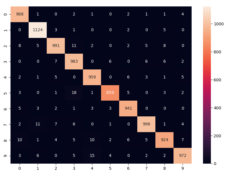
The above confusion matrix provides detailed insight into the model's performance across the ten classes (digits 0 through 9) that the dataset comprises.

Here's a breakdown of how to interpret the matrix:

• The x-axis (horizontal axis) represents the predicted labels that the model has output.
• The y-axis (vertical axis) represents the true labels or the actual classifications of the data.
• Each cell in the matrix represents the count of instances for the actual label (y-axis) that was predicted as a certain label (x-axis).
• The diagonal cells, which run from the top left to the bottom right, show the number of times the model correctly predicted each class. The darker shading and higher numbers along this diagonal indicate more correct predictions.
• Off-diagonal cells indicate misclassifications. For instance, a non-zero value at the location (2, 3) would mean that the model mistakenly predicted some instances of the actual class '2' as class '3'.
• The color intensity and the number in each cell correspond to the count of predictions. Darker or more intense colors represent higher counts. In this case, a gradient from light to dark shades is used, with light representing fewer instances and dark representing more.

Looking at the matrix, we can make a few observations:

• The model has high accuracy for most digits, as indicated by the high counts in the diagonal cells (e.g., 968 for '0', 1124 for '1', etc.).
• Some misclassifications are evident for nearly every digit but are relatively low in number compared to the correct predictions.
• The model seems particularly accurate with digits such as '1' and '7', given the high count and the fact that there are fewer off-diagonal numbers in these rows and columns.

In summary, this Confusion Matrix is a useful visualization to evaluate the model's performance, indicating not only how often it is correct but also what types of errors it's making.

Code

In this section we will go through the code used to train the model.

Imports && Magic Numbers

import os
from pathlib import Path
from typing import Final

import tensorflow as tf

import utils

This block imports necessary Python modules and TensorFlow, which is the core library for creating and training neural networks. The utils module is likely a custom utility library for logging and other functions.

EPOCHS: Final[int] = 4

EPOCHS in the context of the provided code refers to a constant value that defines the number of times the entire training dataset is passed forward and backward through the neural network. The term is a key concept in the training of machine learning models, especially neural networks.

Load model

utils.log_to_file(f"Training with EPOCHS={EPOCHS}")

"""minst.load_data()
Returns:
    - Tuple of NumPy arrays: (x_train, y_train), (x_test, y_test).

    - x_train: uint8 NumPy array of grayscale image data with shapes
    (60000, 28, 28), containing the training data. Pixel values range from 0 to 255.

    - y_train: uint8 NumPy array of digit labels (integers in range 0-9)
    with shape (60000,) for the training data.

    - x_test: uint8 NumPy array of grayscale image data with shapes
    (10000, 28, 28), containing the test data. Pixel values range from 0 to 255.

    - y_test: uint8 NumPy array of digit labels (integers in range 0-9)
    with shape (10000,) for the test data.
"""

minst = tf.keras.datasets.mnist
(x_train, y_train), (x_test, y_test) = minst.load_data(path=os.path.join(
    utils.DATA_DIR, 
    "datasets", 
    "mnist.npz"
))

This snippet loads the MNIST dataset, which contains images of handwritten digits and their corresponding labels, separating it into training and test sets.

assert x_train.shape == (60_000, 28, 28)
assert x_train.dtype == "uint8"

assert y_train.shape == (60_000,)
assert y_train.dtype == "uint8"

assert x_test.shape == (10_000, 28, 28)
assert x_test.dtype == "uint8"

assert y_test.shape == (10_000,)
assert y_test.dtype == "uint8"

The assert statements validate the dimensions and data types of the training and test datasets, ensuring data integrity before moving on to training.

Training Model

x_train = tf.keras.utils.normalize(x_train, axis=1)
x_test = tf.keras.utils.normalize(x_test, axis=1)

These lines normalize the image data within the range 0-1, which can lead to improved training efficiency and model convergence. See What is Feature Scaling & Why is it Important in Machine Learning? or All about Feature Scaling.

assert x_train.dtype == "float64"
assert x_test.dtype == "float64"

Post-normalization, these assertions confirm that the data types of the training and test inputs are now floating-point numbers.

model = tf.keras.models.Sequential()
model.add(tf.keras.layers.Flatten(input_shape=(28, 28)))
model.add(tf.keras.layers.Dense(units=128, activation=tf.nn.relu))
model.add(tf.keras.layers.Dense(units=128, activation=tf.nn.relu))
model.add(tf.keras.layers.Dense(units=10, activation=tf.nn.softmax))

model.compile(
    optimizer=tf.keras.optimizers.Adam(), 
    loss=tf.keras.losses.SparseCategoricalCrossentropy(), 
    metrics=['accuracy']
)

The above code segment sets up the neural network architecture. It uses a sequential model with flattened input and dense layers with ReLU activations, culminating in a softmax layer for classification. The model is compiled with the Adam optimizer and sparse categorical crossentropy loss function, focusing on accuracy as the performance metric.

model.fit(x_train, y_train, epochs=EPOCHS)

The model is trained on the preprocessed training data for the number of epochs specified earlier.

model.summary()

Model: "sequential"
_________________________________________________________________
 Layer (type)                Output Shape              Param #   
=================================================================
 flatten (Flatten)           (None, 784)               0         
                                                                 
 dense (Dense)               (None, 128)               100480    
                                                                 
 dense_1 (Dense)             (None, 128)               16512     
                                                                 
 dense_2 (Dense)             (None, 10)                1290      
                                                                 
=================================================================
Total params: 118282 (462.04 KB)
Trainable params: 118282 (462.04 KB)
Non-trainable params: 0 (0.00 Byte)
_________________________________________________________________

A summary of the model's architecture is printed, showing the layers and parameters.

val_loss, val_acc = model.evaluate(x_test, y_test)
utils.log_to_file(f"Loss: {val_loss:.4f}, Accuracy: {val_acc*100:.2f}%")

model_path: Path = os.path.join(
    utils.DATA_DIR, 
    "models", 
    str(EPOCHS), 
    f"mnist-{EPOCHS}-{val_acc*100:.2f}.model"
)
model.save(model_path)

utils.log_to_file(f"Finished training with EPOCHS={EPOCHS}")
utils.log_to_file(f"Model saved to path '{str(model_path)}'")

Calc Confusion Matrix

import numpy as np

y_test_predected: np.ndarray[np.ndarray] = model.predict(x_test)

y_test_predected_labels: list[int] = [
    np.argmax(prediction)
    for prediction in y_test_predected
]

utils.log_to_file(f"False predictions: {sum(y_test_predected_labels != y_test):,}/{len(y_test):,}")
utils.log_to_file(f"True predictions: {sum(y_test_predected_labels == y_test):,}/{len(y_test):,}")

confusion_matrix = tf.math.confusion_matrix(
    labels=y_test,
    predictions=y_test_predected_labels
)

import seaborn as sn
import pandas as pd
import matplotlib.pyplot as plt

plt.figure(figsize=(10,7))
sn.heatmap(confusion_matrix, annot=True, fmt='g')

Path(os.path.join(
    utils.DATA_DIR, 
    "confusion-matrices", 
    str(EPOCHS), 
    "train"
)).mkdir(parents=True, exist_ok=True)

confusion_matrix_path: Path = os.path.join(
    utils.DATA_DIR, 
    "confusion-matrices", 
    str(EPOCHS), 
    "train",
    f"mnist-{EPOCHS}-{val_acc*100:.2f}.png"
)
plt.savefig(confusion_matrix_path)
plt.show()

utils.log_to_file(f"Confusion matrix saved to path '{str(confusion_matrix_path)}'")

Extra Custom Test

Custom Datasets

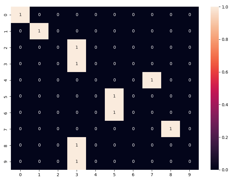
0 predected 0	1 predected 1	2 predected 3	3 predected 3	4 predected 7

5 predected 5	6 predected 5	7 predected 1	8 predected 3	9 predected 3

Confusion Matrix

Wrong Predictions

2 predected 3	4 predected 7	6 predected 5

7 predected 1	8 predected 3	9 predected 3

Logs

[2023-10-25 12:26:40] Training with EPOCHS=4
[2023-10-25 12:26:49] Loss: 0.0918, Accuracy: 97.17%
[2023-10-25 12:26:50] Finished training with EPOCHS=4
[2023-10-25 12:26:50] Model saved to path '/Users/ziadh/Desktop/playgroud/image-processing/classifications/mnist/data/models/4/mnist-4-97.17.model'
[2023-10-25 12:26:50] False predictions: 283/10,000
[2023-10-25 12:26:50] True predictions: 9,717/10,000
[2023-10-25 12:26:50] Confusion matrix saved to path '/Users/ziadh/Desktop/playgroud/image-processing/classifications/mnist/data/confusion-matrices/4/train/mnist-4-97.17.png'
[2023-10-25 17:23:24] Testing model with EPOCHS: 4 and ACCURACY: 97.17
[2023-10-25 17:23:24] predected: 3 and it was 8
[2023-10-25 17:23:24] predected: 3 and it was 9
[2023-10-25 17:23:24] predected: 7 and it was 4
[2023-10-25 17:23:24] predected: 5 and it was 5
[2023-10-25 17:23:24] predected: 1 and it was 7
[2023-10-25 17:23:24] predected: 5 and it was 6
[2023-10-25 17:23:24] predected: 3 and it was 2
[2023-10-25 17:23:24] predected: 3 and it was 3
[2023-10-25 17:23:24] predected: 1 and it was 1
[2023-10-25 17:23:24] predected: 0 and it was 0
[2023-10-25 17:23:24] Accuracy: 40.0%
[2023-10-25 17:23:24] Number of faults: 6/10
[2023-10-25 17:23:24] Number of correct: 4/10

Comments

• We can infer from the confusion matrix and comparing pictures of wrong predictions with correct ones that the model would have been more accurate if skeletonization were performed on the images.

Look up difference between Thinning and skeletonization

REFERENCES

• Repository Containing all the work.
• 3b1b Neural networks
• Stanford CS231n.
• Neural Network Python Project - Handwritten Digit Recognition.