Quick Review
A picture is worth a thousand words.By Fred R. Barnard.
Semantic Gap
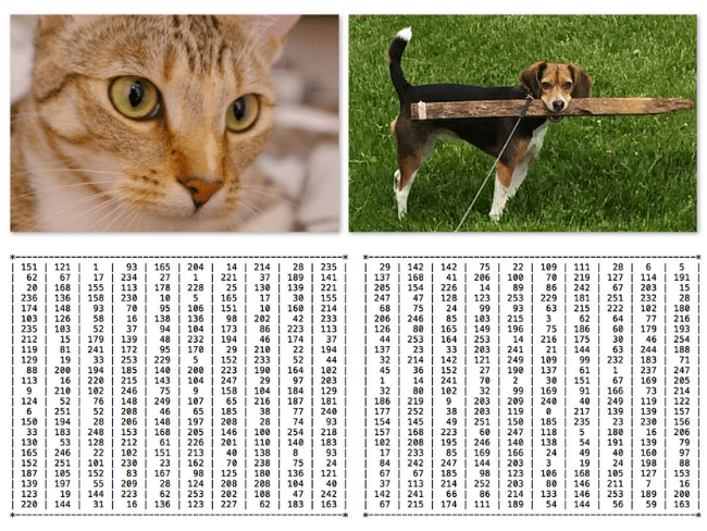
Remember our computer sees is a big matrix of numbers. It has no idea regarding the thoughts, knowledge, or meaning the image is trying to convey.
| Original | What Computer Sees |
|---|---|
 |  |
Definition
Image classification, at its very core, is the task of assigning a label to an image from a predefined set of categories.
Main goal is to process input image and return a label that identifies the image. From a predefined set of categories.
Challenges
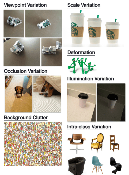
The above image showcases various challenges in image classification due to the differences in how objects may be presented. These challenges include changes in perspective, object size, shape distortion, varying levels of visibility, diverse backgrounds, fluctuations in lighting, and differences within the same object category. These variations highlight the importance of designing robust image classification systems that can accurately recognize objects despite these changes. The system must be adept at understanding objects from different angles, in various light conditions, when they are partially hidden, across a range of sizes, amidst chaotic backgrounds, and even when the objects themselves vary in appearance.
Viewpoint Variations
Initially, there is the challenge of viewpoint variation, which involves the object being presented at different orientations or rotations within the three-dimensional space as it is photographed. Regardless of the perspective from which the Raspberry Pi is imaged, it remains identifiable as a Raspberry Pi.
Scale Variation
It's crucial to factor in the variability in size as well. Take Starbucks coffee cups as an example: whether it's a tall, grande, or venti, they are all variations of a coffee cup, just in different sizes. Moreover, a venti cup's appearance can change significantly depending on whether it's shot from a close distance or a far one. Our image classification techniques need to be resilient to such scale differences.
Deformation
Deformation is among the toughest variations to address. Consider Gumby from the namesake TV series; the character can bend and stretch into a multitude of forms. The various poses of Gumby represent object deformation – the character remains constant, yet each representation appears markedly different.
Occlusion Variation
Our classification algorithms must also handle instances where key parts of the target object are obscured or hidden, as shown with the images of the dog. In one image, the dog is fully visible, while in the other, it's partly concealed under a cover. Despite the occlusion, an effective image classification system should still recognize the dog in both situations.
Illumination Variation
Adjusting for changes in lighting is equally essential. For instance, the same coffee cup looks drastically different under normal lighting compared to dim lighting. Note how certain details, like the cup's cardboard seam, are more apparent in reduced lighting. Our systems need to reliably identify objects across such variations in illumination.
Background Clutter
We should also be prepared for background clutter, which can be likened to the challenge of finding Waldo in the popular search-and-find books. The chaotic scenes in "Where's Waldo?" exemplify how difficult it can be to locate a single object amidst a busy backdrop. This task can be even more daunting for a computer that lacks human-like semantic comprehension.
Intra-class Variation
Finally, we have the challenge of intra-class variation, well-exemplified by the diverse types of chairs. From cozy reading nooks to kitchen seats to high-end art deco furniture, all these are recognized as chairs. Our classification systems need to be adept at categorizing such a broad spectrum of items within the same category.
Multiple Variations Combined
In reality, these variations are often combined. For instance, a coffee cup can be presented at different scales, from different viewpoints, and under varying lighting conditions. The cup can also be occluded by other objects, and it can be placed against a cluttered background.
Our classification systems must be able to handle such combinations of variations.
Strategies for Effective Image Classification
In the field of computer vision and machine learning, the groundwork for a successful application begins with setting precise and realistic objectives. If one aims too high at the outset, for instance, by aspiring to classify every plant species in a garden, the complexity could become overwhelming, possibly leading to suboptimal results without a deep reservoir of expertise and extensive data.
On the other hand, if you target a more specific goal, such as distinguishing between just roses and tulips, you set up a manageable framework that enhances the chances of accuracy and reliability, an ideal approach for those just starting with image recognition.
The essential advice is to craft a well-bounded and concise mission for your image recognition endeavor. Despite the impressive capabilities of advanced neural networks to tackle various difficulties, it is beneficial to delineate the project's scope with precision and clarity for the most effective outcomes.
Important Concepts
The following concepts are essential to understand before we dive into the details of image classification. And will help you boost efficiency of your image classification model.
Data augmentation
Data augmentation is a technique to artificially create new training data from existing training data.
Data augmentation is a strategy used to increase the diversity of data available for training models without actually collecting new data. This technique involves making systematic modifications to existing data samples to create new samples with the same labels. The idea is to expose the model to a wider array of variations during training, which helps improve the model's generalization abilities when it encounters new, unseen data.
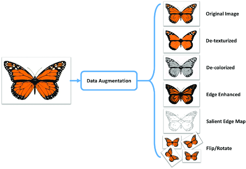
The images provided illustrate several common data augmentation techniques:
In the first image, a butterfly's photograph undergoes various transformations. The original image is used to generate additional variations through processes like de-texturizing, which simplifies the texture; de-colorizing, which removes color information; and edge enhancement, which highlights the edges in the image. There's also a salient edge map that outlines the most prominent edges, and the image is manipulated through flips and rotations to simulate different orientations.
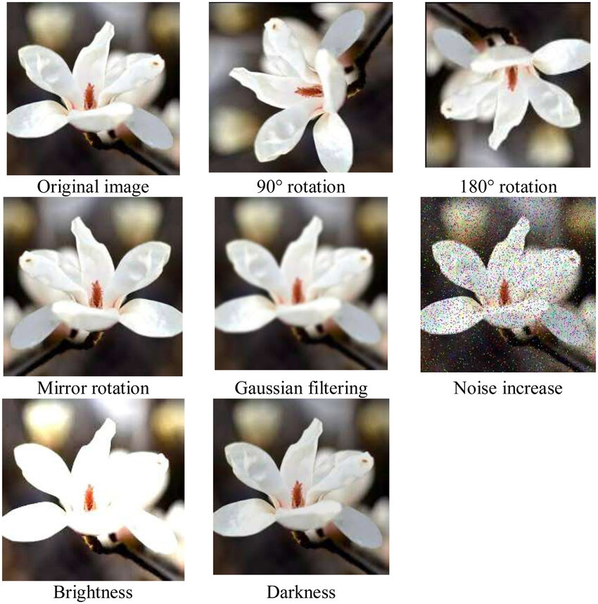
The second image showcases a flower subjected to different transformations: rotating by 90 and 180 degrees to change the orientation, mirror rotation to reflect the image, Gaussian filtering to blur, and adding noise to simulate a grainy effect. Adjustments in brightness and darkness are also demonstrated to account for changes in illumination.
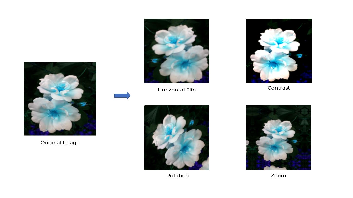
The third image depicts a flower that has been horizontally flipped, rotated, zoomed, and had its contrast altered. These changes mimic how the subject might be captured from different angles or under different photographic conditions.
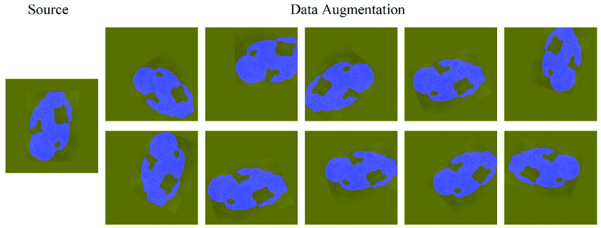
The fourth image sequence shows a blue object against a green background. This object is presented with variations in its position and orientation within the frame, simulating different perspectives from which it might be viewed.
By using data augmentation techniques like these, a machine learning model can learn to recognize objects regardless of changes in viewpoint, scale, lighting, or background. It's a fundamental step in creating robust image recognition systems that need to perform well in varied real-world conditions. Data augmentation is especially useful when the amount of original data is limited, as it artificially expands the dataset size and variety, leading to improved model performance.
Confusion Matrix
A Confusion Matrix is a powerful tool used in machine learning for measuring the performance of classification algorithms. It's especially useful when the classification problem is binary (two classes) or multiclass (more than two classes).
Here's how a Confusion Matrix works:
True Positives (TP): The cases in which the model correctly predicts the positive class.True Negatives (TN): The cases in which the model correctly predicts the negative class.False Positives (FP): The cases in which the model incorrectly predicts the positive class. This is also known as a Type I error.False Negatives (FN): The cases in which the model incorrectly predicts the negative class. This is also known as a Type II error.
The Confusion Matrix is laid out as a table with two dimensions: "Actual" and "Predicted." Each row of the matrix represents the instances in a predicted class, while each column represents the instances in an actual class. Here's a simple layout:
| Predicted Positive | Predicted Negative | |
|---|---|---|
| Actual Positive | True Positive (TP) | False Negative (FN) |
| Actual Negative | False Positive (FP) | True Negative (TN) |
From the Confusion Matrix, various metrics can be calculated to evaluate the performance of a classification model:
Accuracy: The ratio of correctly predicted instances to the total instances in the dataset.Precision: The ratio of correctly predicted positive observations to the total predicted positive observations. It is also known as the Positive Predictive Value.Recall or Sensitivity: The ratio of correctly predicted positive observations to all the actual positives. It is also known as the True Positive Rate.F1 Score: The weighted average of Precision and Recall, used when you seek a balance between Precision and Recall.Specificity: The ratio of correctly predicted negative observations to all the actual negatives.
By analyzing the Confusion Matrix, one can gain insight into not only the performance of the model but also which classes are being confused with each other, which can inform further refinement of the classifier. It's an indispensable part of model evaluation in supervised learning tasks.
Epochs
The EPOCHS value is a critical hyperparameter in training neural networks, as it directly impacts the model's ability to learn from the training data.
- When training a model, one epoch consists of one complete cycle of passing all the training data through the neural network and then running a backpropagation algorithm to update the weights. This process is aimed at minimizing the loss function, which measures the difference between the model's predictions and the actual values.
- The EPOCHS: Final[int] = 4 line sets the number of epochs as a constant to the value of 4, indicating that the dataset will be used in four complete cycles of forward and backward passes during the training process.
- The use of the Final type hint from the typing module suggests that the value of EPOCHS is intended to remain unchanged throughout the program, making it a constant. This is often done to avoid magic numbers in the code and to provide clear, configurable parameters at the top of the script.
- In practical terms, setting the number of epochs is a balancing act. Too few epochs might result in an underfit model that does not learn enough from the data, while too many epochs can lead to overfitting, where the model learns the training data too well, including its noise and outliers, which can negatively affect performance on unseen data.